Unit 24 - MODIS
The Moderate Resolution Imaging Spectroradiometer (MODIS) is a 36-channel from visible to thermal-infrared sensor that was launched as part of the Terra satellite payload in December 1999 and Aqua satellite in May 2002. The Terra satellite passes twice a day (at 10:30am and 22:30pm local time), the Aqua satellite also passes twice a day (at 01:30am and 13:30pm local time). (source: GRASS Wiki)
Our area of interest, Germany, is covered by two MODIS tiles (see MODLAND grid):
h18v03
h18v04
MODIS data is provided in 3 projections (Sinusoidal, Lambert Azimuthal Equal-Area, and Geographic). For our purpose, data will be reprojected to ETRS89 / LAEA Europe EPSG:3035.
Create a new GRASS project germany-modis (see Unit 02) using EPSG code (Select CRS from a list by EPSG or description).
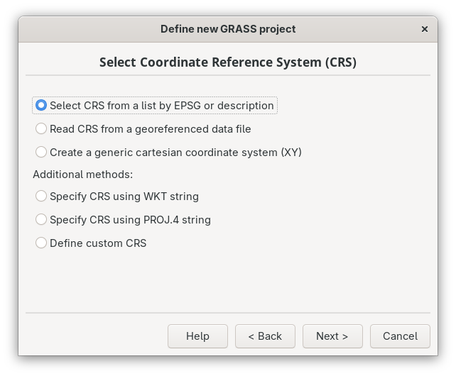
Fig. 112 Create a new project based on EPSG code.
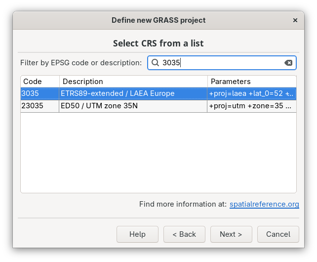
Fig. 113 Enter EPSG code.
Enter a new GRASS session (PERMANENT mapset) and install i.modis addons extension (more about installing addons in Unit 17) for downloading and importing MODIS data (note that you have to install also pyMODIS Python Library). Run two commands below in Console tab.
python3 -m pip install setuptools slugify pymodis

g.extension extension=i.modis
GRASS MODIS addon consists of two tools:
Download data
Important
Pre-downloaded MODIS data (year 2023) is available in the
sample dataset (modis directory). Readers can continue with
importing sample data.
Let’s download desired tiles (h18v03 and h18v04) for year 2023 by i.modis.download.
Land Surface Temperature eight day 1 Km (Terra/Aqua) product will be downloaded.
i.modis.download settings=settings.txt folder=modis \
tiles=h18v03,h18v04 \
product=lst_aqua_eight_1000,lst_terra_eight_1000 \
startday=2023-01-01 endday=2023-12-31
Note
Output folder (h18v03_04 in this case) must exists,
otherwise the tool will fail.
File settings.txt contains two lines: username and
password for accessing MODIS download service.
Please read pyModis documentation how to register and set up your account.
Import data
Input MODIS data can be imported and reprojected into target project by i.modis.import.
i.modis.import -qmw files=modis/listfileMOD11A2.061.txt outfile=tlist-mod.txt

i.modis.import -qmw files=modis/listfileMYD11A2.061.txt outfile=tlist-myd.txt
If -m flag is given mosaic from input tiles is created
automatically, see Fig. 114.
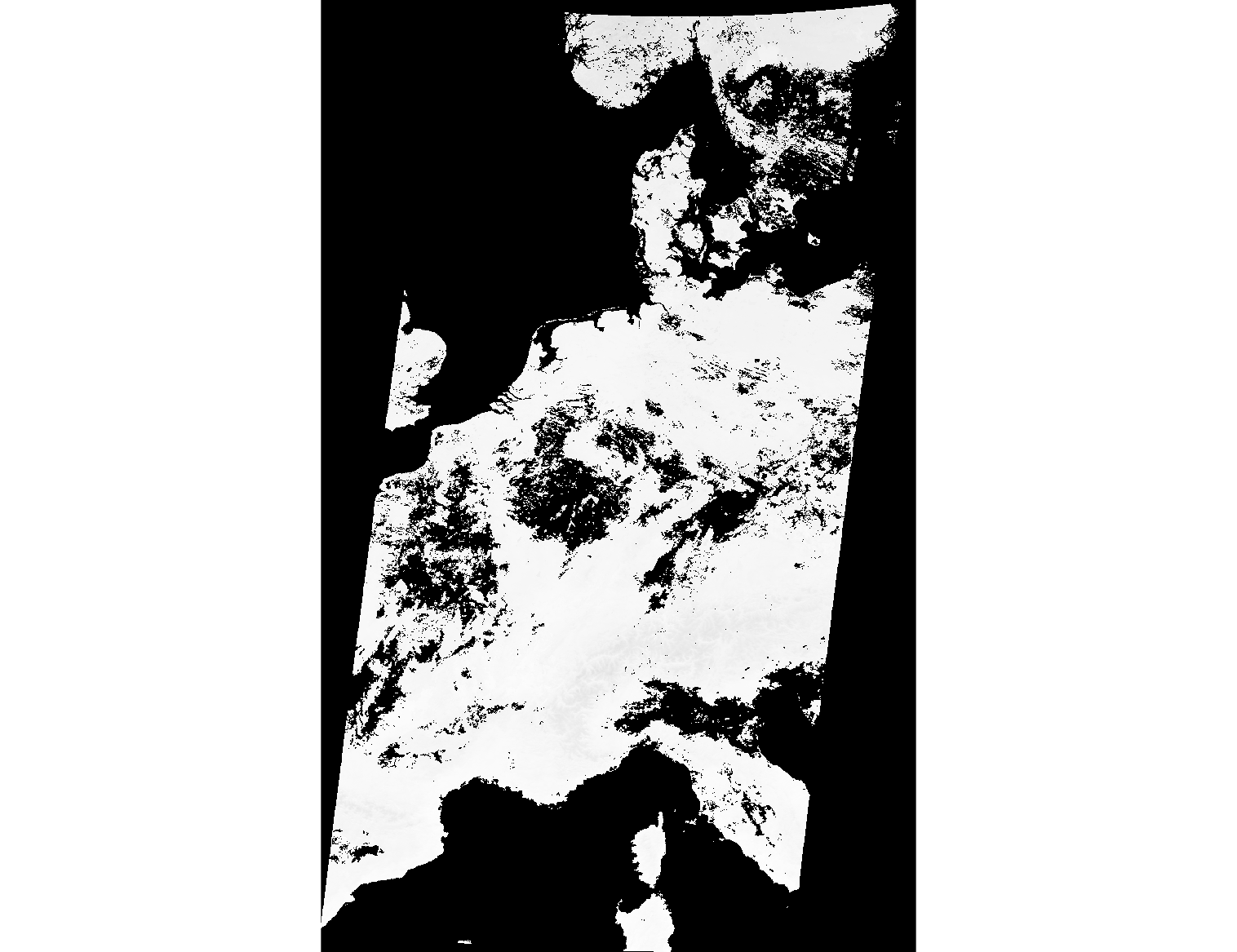
Fig. 114 Data mosaic created from h18v03 and h18v04 tiles.
Germany administrative border
Germany administrative border can created by dissolving
counties used in Unit 14 - PyGRASS Vector Access. Let’s import
osm/counties.gpkg into the current GRASS project as described
in Unit 03 - Data Management.
Next, open the attribute table  Show attribute data
for selected vector map and add a new column used for dissolving.
Show attribute data
for selected vector map and add a new column used for dissolving.
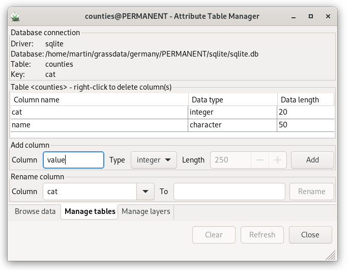
Fig. 115 Add a new column ‘value’.
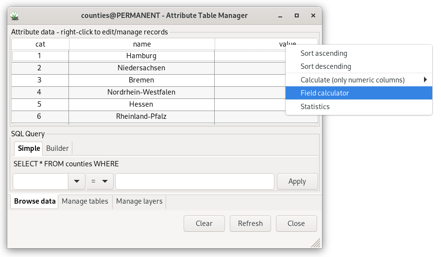
Fig. 116 Open Field calculator.
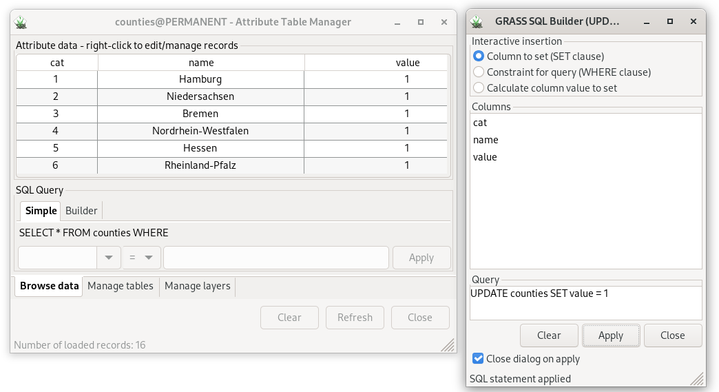
Fig. 117 Fill new column by value of 1.
Tip
Steps described above may me performed from command line by v.db.addcolumn and v.db.update.
v.db.addcolumn map=counties columns="value int"
v.db.update map=counties column=value value=1
Now, we can perform dissolving all counties by v.dissolve:
v.dissolve input=counties output=germany column=value
LST
In this section Land Surface Temperature (LST) analysis will be perfmored for Germany.
Mask will be created by r.mask. Don’t forget that computational region must be set before creating a mask. Computational region will be defined by Germany vector map and aligned by the input MODIS data by g.region.
g.region vector=germany align=MOD11A2.A2023001_mosaic_LST_Day_1km
r.mask vector=germany
Let’s check range values of imported MODIS data by r.info tool:
r.info -r map=MOD11A2.A2023001_mosaic_LST_Day_1km
min=0
max=14511
In order to determine LST from input data, digital values (DN) must be converted into Celsius or Kelvin scale.
Conversion to Celsium scale can be done by r.mapcalc (see also Unit 05 - Raster processing). It’s also suitable to replace zero values with no-data value (NULL value in GRASS terminology).
r.mapcalc expression="MOD11A2.A2023001_mosaic_LST_Day_1km_c = \
if(MOD11A2.A2023001_mosaic_LST_Day_1km != 0, \
MOD11A2.A2023001_mosaic_LST_Day_1km * 0.02 - 273.15, null())"
Let’s check range values of new LST data layer.
r.info -r map=MOD11A2.A2023001_mosaic_LST_Day_1km_c
min=-22.21
max=12.09
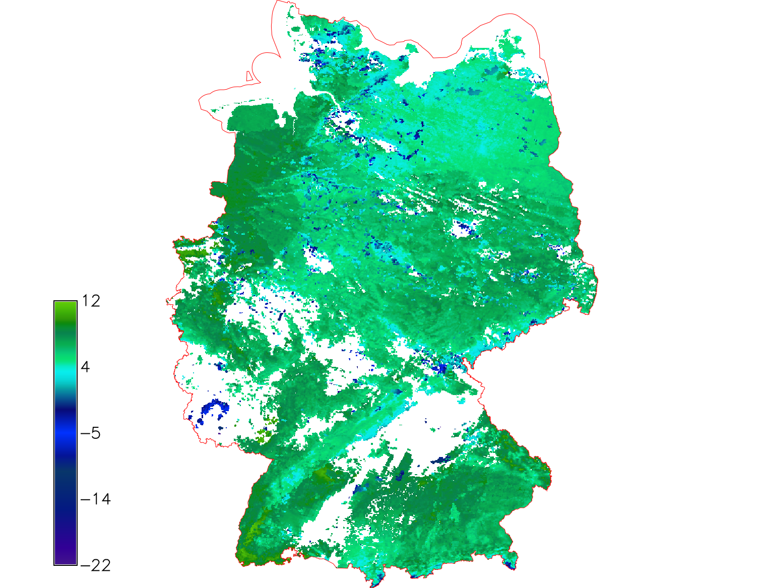
Fig. 118 LST reconstruction for Germany in Celsius scale (color table
celsius applied).