Unit 02 - First steps

Starting a GRASS session requires basic knowledge about the software itself. GRASS motivates users to organize their data from an early beginning. GRASS uses a consistent structure of so-called locations and mapsets to organize its data. This has not changed in GRASS 8.

The GRASS data structure has three levels:

1. Database directory. A directory on local or network disc which contains all data accessed by GRASS. It’s usually a directory called grassdata located in users’ home directory.

2. Location. All geodata stored within one location must have the same spatial coordinate system (GRASS doesn’t support on-the-fly projection for several reasons).

3. Mapset. Contains task-related data within one project. Helps organizing data into logical groups or to separate parallel work of different users on the same project.

Note

In GRASS 7, a startup screen (Fig. 3) appeared before entering a session. The user had to define the working environment in which the GRASS session started. This step was required to enter GRASS. Such an approach is not so common. Applications like Esri ArcGIS or QGIS just start. Users load different data from various sources in different projections and start working on their project.

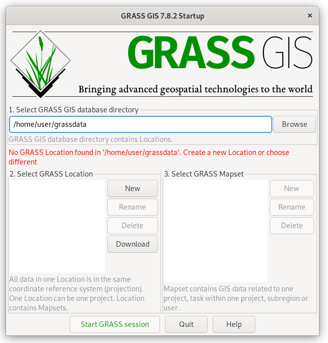
Fig. 3 GRASS GIS startup screen in version 7.

Obstacles (especially for newcomers) related to the startup screen have been reduced in GRASS 8. The startup screen has been replaced by a completely new mechanism. On the first launch, GRASS 8 sets up the database directory automatically and launches GUI in a default location World LatLong WGS84. Also, a sample world vector layer (in GRASS terminology vector map) is shown.

GRASS GUI is designed as a simple and lightweight graphical user interface. Basically, it is a GUI front-end calling GRASS commands (see Accessing GRASS modules) in the background. The GUI consists of two main windows, see Fig. 4.

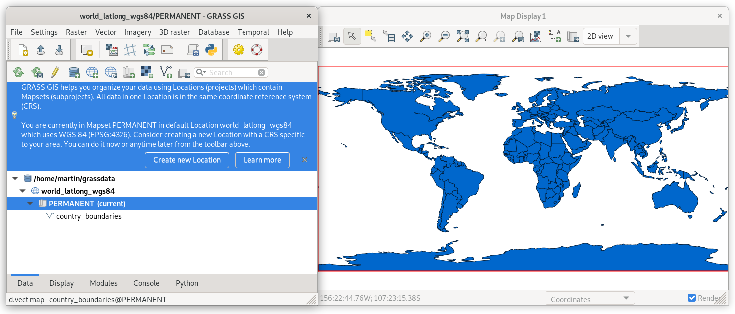
Fig. 4 GRASS GIS 8 on startup.

Tip

If GUI crashes, it can be started again by g.gui command from the underlying terminal (command prompt).

GRASS GUI guides users by means of tooltips as shown in Fig. 4. The default location is not designed for real work. The next step is usually to create new “project(s)” (in GRASS terminology a location) with user-defined spatial coordinate systems.

Note

Consider changing language settings to English in Settings ‣ Preferences ‣ Appearance. Change Language settings to en and restart GRASS.

Create a new location

By clicking on Create new Location button in the tooltip (or by from the toolbar) the wizard appears. A new GRASS location can be easily created using EPSG codes or user-defined geodata.

In the first page of the location wizard, the location name is defined. Optionally, also a short description can be added.

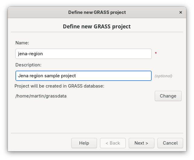
Fig. 5 Define a name for the new GRASS location.

In the next page, a coordinate reference system (CRS) is chosen. CRS is usually defined by EPSG code (Select CRS from a list by EPSG or description) or by user-defined geodata (Read CRS from a georeferenced data file).

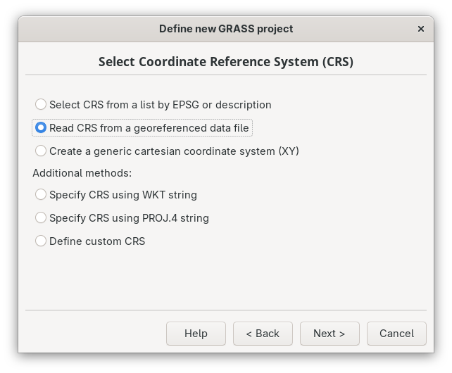
Fig. 6 Choose “Read CRS from a georeferenced data file” for creating a new GRASS location.

In our case, a new location will be created by defining CRS from jena_boundary.gpkg input file (located in the sample dataset in osm directory).

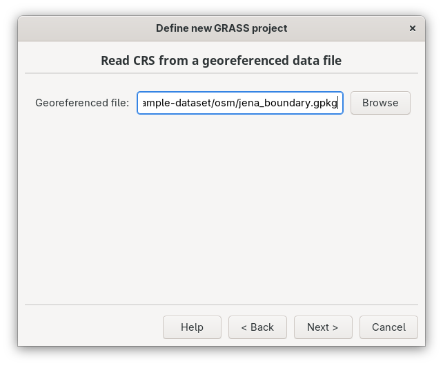
Fig. 7 Define an input file jena_boundary.gpkg.

Note

Jena administrative boundary has been downloaded from OSM using Overpass API.

(
relation["boundary"="administrative"]
    ["admin_level"="6"]
    ["name"="Jena"];
);
(._;>;);
out body;

Exported GeoJSON file has been converted to GeoPackage (and reprojected to UTM zone 32N (EPSG:32632) since we want to work with Sentinel data afterwards, see Unit 03 - Data Management) by GDAL ogr2ogr utility:

ogr2ogr -f GPKG -dialect SQLite \
-sql "select * from export where st_geometrytype(geometry) IN ('POLYGON', 'MULTIPOLYGON')" \
-nln jena_boundary -t_srs EPSG:32632 jena_boundary.gpkg export.geojson

Spatial reference system is chosen based on input file (UTM zone 32N EPSG:32632).

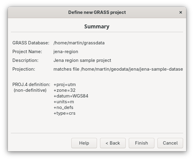
Fig. 8 Check the summary.

A new GRASS user-defined location will be created by clicking on Finish button.

After creating a new location (Finish button) the user can optionally import data used for defining the new location (in our case jena_boundary.gpkg).

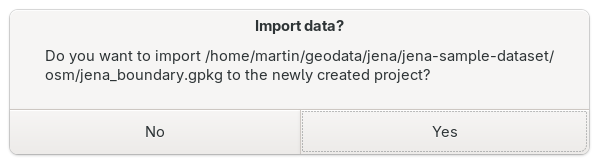
Fig. 9 Let’s import data to simplify our first steps in GRASS GIS.

By default GRASS creates a PERMANENT mapset in the new location. Here, all location settings are stored. This mapset is commonly used for importing input geodata used in the location.

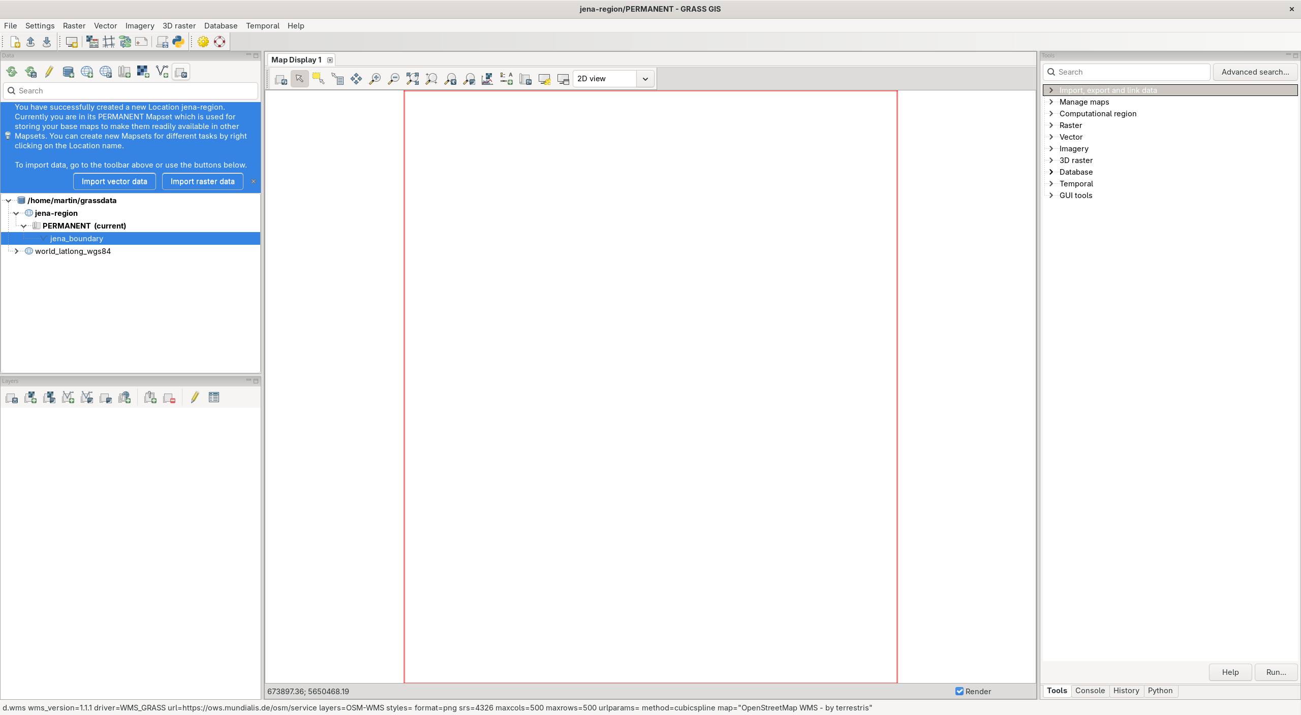
Fig. 10 GRASS GUI automatically switches to the new location.

Display data

Imported jena_boundary data layer can be easily displayed from Data tab.

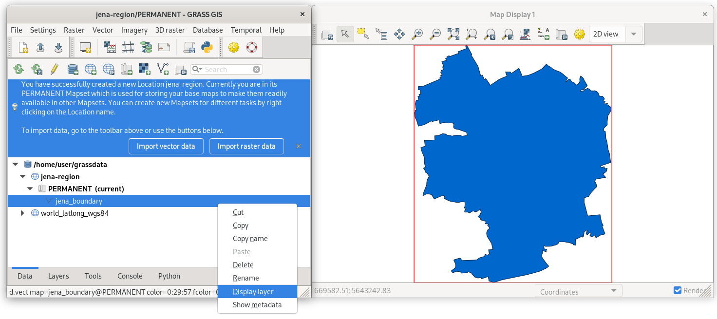
Fig. 11 Display Jena city administrative boundary vector layer. Select Display layer from contextual menu in Data tab or simply use double-click on the specified layer.

Let’s also add a basemap from freely available OpenStreeMap map service. In our case OpenStreetMap WMS provided by mundialis company (http://ows.mundialis.de/services/service). WMS layer can be added from Layers tab ^{Add web service layer}.

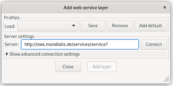
Fig. 12 Connect to the defined WMS server.

After connecting to the WMS server, desired layer can be chosen.

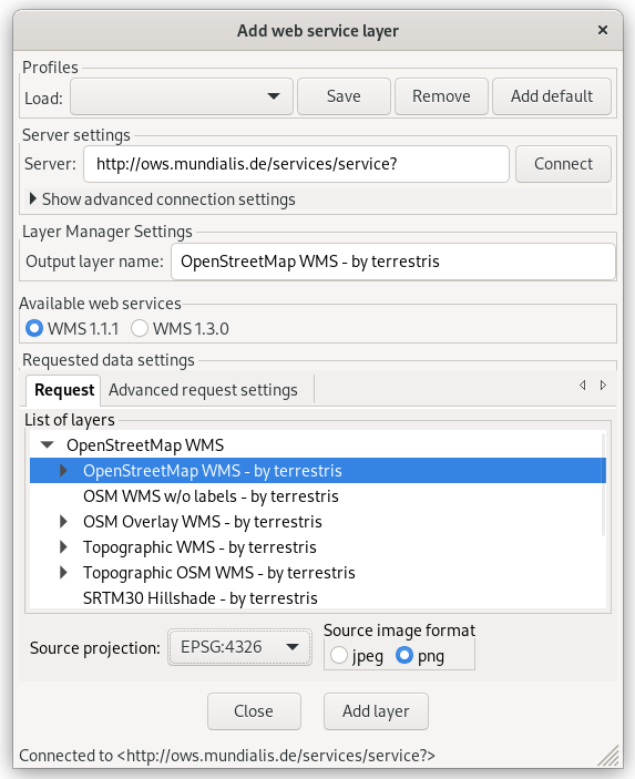
Fig. 13 Choose WMS layer to be displayed.

In Layers tab change order of layers (move jena-boundary on the top) and tune display properities of jena-boundary layer.

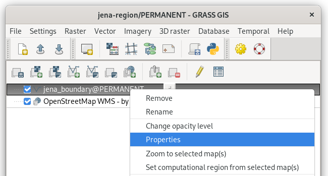
Fig. 14 Choose Properties from contextual menu (right click on selected layer).

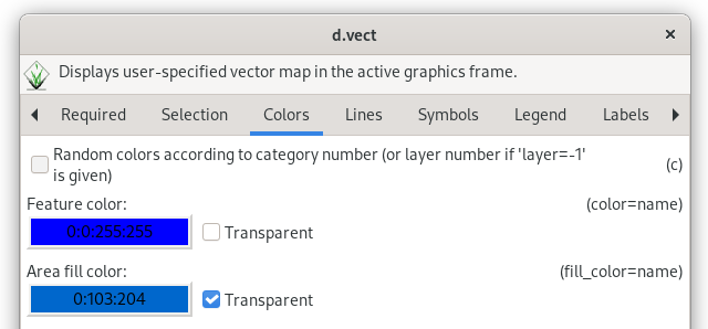
Fig. 15 Change map layer properties: outline in blue color, fill color transparent.

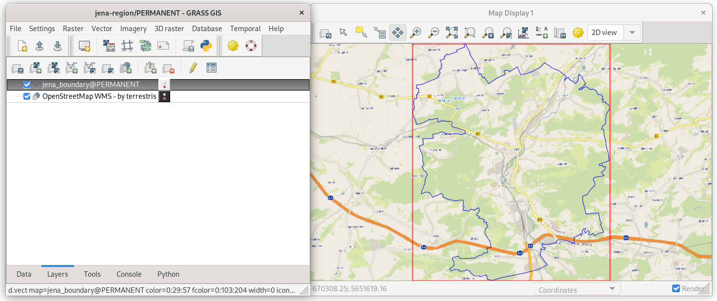
Fig. 16 A map composition of basemap and boundary of Jena city region in blue color.