Unit 21 - Sentinel spatio-temporal

Create a new mapset in jena-region location: sentinel_st.

Important

Do not use dashes in the mapset name otherwise t.rast.algebra will most probably fail.

Download data

Important

Pre-downloaded Sentinel scenes are available in the sample dataset (directory sentinel/2019). Readers can continue with importing sample data.

Let’s download Sentinel L2A products for spring/summer 2021. There are 6 products available as shown below.

i.sentinel.download -l settings=sentinel.txt map=jena_boundary area_relation=Contains \
start=2021-04-01 end=2021-10-31 producttype=S2MSI2A clouds=10

6 Sentinel product(s) found
a844500a-049f-46a3-92de-bcda2c38fc3c ... 2021-05-31T10:15:59Z  2% S2MSI2A 1.09 GB
d5b73db9-0acf-401d-9bf4-a6f199df1119 ... 2021-09-08T10:15:59Z  3% S2MSI2A 1.09 GB
b00d5dfd-9cce-48c6-a011-fd46b85de814 ... 2021-09-03T10:20:21Z  3% S2MSI2A 1.09 GB
44644895-f6f9-4963-ab47-b5e122d3bf41 ... 2021-08-14T10:20:31Z  5% S2MSI2A 1.10 GB
dc92df2b-b69e-4081-88a6-bd4b95e4fc78 ... 2021-04-21T10:15:49Z  8% S2MSI2A 1.08 GB
2c02ac80-60ae-4376-9099-2267ad3a96b5 ... 2021-04-26T10:20:21Z  9% S2MSI2A 1.09 GB

Download selected Sentinel scenes:

i.sentinel.download settings=sentinel.txt map=jena_boundary area_relation=Contains \
start=2021-04-01 end=2021-10-31 producttype=S2MSI2A clouds=10 \
output=geodata/sentinel/2021

Import data

Data can be imported by i.sentinel.import similarly as done in Unit 20 - Sentinel downloader. At fisrt check list of bands to be imported by -p flag. Since NDVI is computed only 4th and 8th band are selected. Use register_output in order to create timestamps file. This file will be used for registering bands into space-time raster dataset.

i.sentinel.import -p input=geodata/sentinel/2019 pattern="B0[4|8]_10m"

i.sentinel.import -l -c input=geodata/sentinel/2019 pattern="B0[4|8]_10m" \
register_output=sentinel-timestamps.txt

Example of created timestamp file:

T32UPB_20190407T102021_B04_10m|2019-04-07 10:26:45.035007|S2_4
T32UPB_20190407T102021_B08_10m|2019-04-07 10:26:45.035007|S2_8
T32UPB_20190422T102029_B04_10m|2019-04-22 10:26:50.312683|S2_4
...

Create space-time dataset

At this moment a new space-time dataset can be created by means of t.create and all imported Sentinel bands registered with t.register.

t.create output=sentinel title="Sentinel L2A 2019" desc="Jena region"
t.register input=sentinel file=sentinel-timestamps.txt

Let’s check basic metadata (t.info) and list the registered maps (t.rast.list).

t.info input=sentinel

...
| Start time:................. 2019-04-07 10:26:45.035007
| End time:................... 2019-10-14 10:26:46.742599
...
| Semantic labels:............ S2_4,S2_8
| Number of registered maps:.. 14

t.rast.list input=sentinel

name|mapset|start_time|end_time
T32UPB_20190407T102021_B04_10m|sentinel_ndvi|2019-04-07 10:26:45.035007|None
T32UPB_20190407T102021_B08_10m|sentinel_ndvi|2019-04-07 10:26:45.035007|None
T32UPB_20190417T102031_B04_10m|sentinel_ndvi|2019-04-17 10:26:46.415802|None
...

NDVI ST computation

For NDVI computation 4th and 8th bands are required (Unit 05 - Raster processing). Map algebra for spatio-temporal data is performed by t.rast.algebra which requires bands separated into different spatio-temporal datasets (see example in Unit 22 - Spatio-temporal scripting). Such datasets can be prepared by t.rast.extract.

t.rast.extract input=sentinel where="semantic_label = 'S2_4'" output=b4
t.rast.extract input=sentinel where="semantic_label = 'S2_8'" output=b8

Let’s check content of the new datasets by t.rast.list using semantic labels.

t.rast.list input=b4
t.rast.list input=b8

Set computational region by g.region including mask for area of interest by r.mask.

g.region vector=jena_boundary align=T32UPB_20190407T102021_B04_10m
r.mask vector=jena_boundary

NDVI (see Unit 05 - Raster processing) computation on spatio-temporal datasets can be performed in parallel (nproc).

t.rast.algebra basename=ndvi expression="ndvi = float(b8 - b4) / ( b8 + b4 )" nprocs=3

Tip

GRASS 8 adds mechanism of semantic labels which makes computation much more straighforward using t.rast.mapcalc. NDVI can be computed directly using sentinel space-time dataset. No need for creating time series subsets as described above.

t.rast.mapcalc inputs=sentinel.S2_8,sentinel.S2_4 output=ndvi basename=ndvi \
expression="float(sentinel.S2_8 - sentinel.S2_4) / (sentinel.S2_8 + sentinel.S2_4)" \
nprocs=3

When computation is finished ndvi color table can be set with t.rast.colors.

t.rast.colors input=ndvi color=ndvi

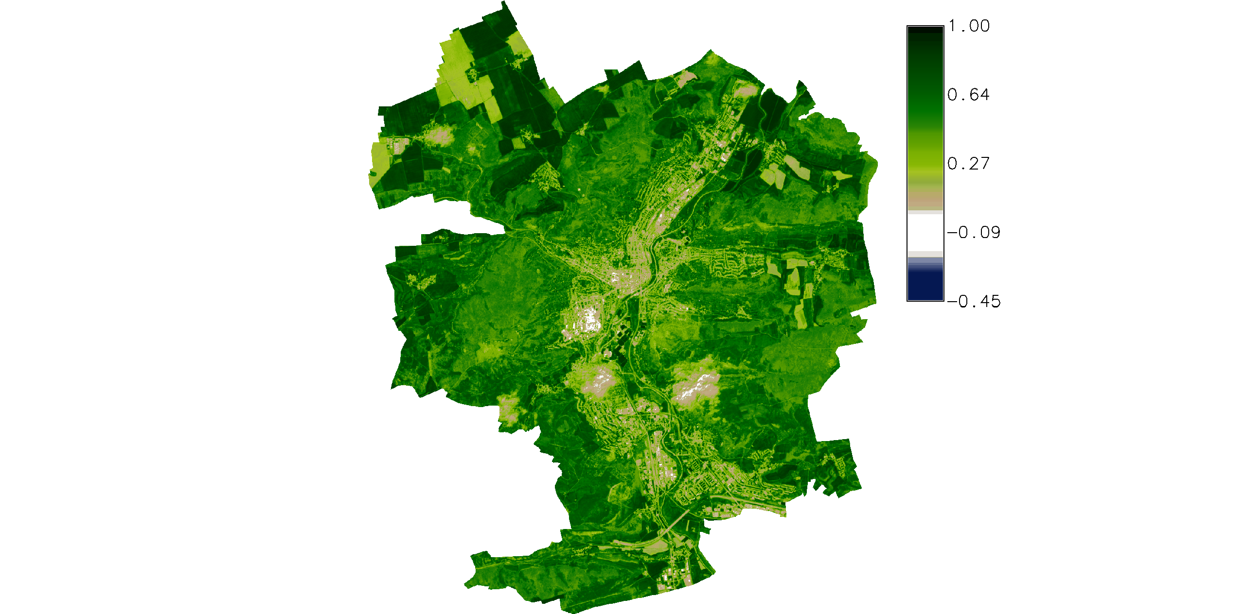
Fig. 109 Simple NDVI animation (no clouds mask applied) created by g.gui.animation.

Important

Load data as multiple raster maps instead of space time dataset.

Cloud mask

Let’s apply the cloud masks on our NDVI space-time dataset. At first, we will create a new space-time dataset containing computed raster masks. A sample Python script has been designed for this purpose below. In case the scene contains clouds (43), a vector mask is created (44), which is then rasterized using v.to.rast (48).

#!/usr/bin/env python3

# %module
# % description: Creates raster mask maps based on clouds mask features.
# %end
# %option G_OPT_V_MAP
# % description: Name of AOI vector map
# %end
# %option G_OPT_STRDS_INPUT
# % description: Name of input 4th band space time raster dataset
# %end
# %option G_OPT_F_OUTPUT
# %end

import sys

import grass.script as gs

from grass.pygrass.gis import Mapset
from grass.pygrass.modules import Module
from grass.pygrass.vector import VectorTopo
from grass.pygrass.utils import copy
import grass.temporal as tgis

def main():
    mapset = Mapset()
    mapset.current()

    tgis.init()
    sp4 = tgis.open_old_stds(options['input'], 'raster')
    
    with open(options['output'], 'w') as fd:
        for t_item in sp4.get_registered_maps(columns='name,start_time'):
            items = t_item[0].split('_')
            d = t_item[1]

            vect = '{}_{}_MSK_CLOUDS'.format(items[0], items[1])
            mask_vect = '{}_{}'.format(vect, options['map'].split('@')[0])
            n_clouds = 0
            with VectorTopo(vect) as v:
                if v.exist():
                    n_clouds = v.num_primitive_of('centroid')
            if n_clouds > 0:
                Module('v.overlay', ainput=options['map'], binput=vect, operator='not',
                       output=mask_vect, overwrite=True)
            else:
                copy(options['map'], mask_vect, 'vector')
            Module('v.to.rast', input=mask_vect, output=mask_vect, use='value', overwrite=True)
            Module('g.remove', flags='f', type='vector', name=mask_vect)
            fd.write("{}|{}\n".format(
                mask_vect,
                d.strftime('%Y-%m-%d %H:%M:%S.%f'),
            ))
        
    return 0

if __name__ == "__main__":
    options, flags = gs.parser()
    
    sys.exit(main())

Sample script to download: sentinel-cloud-mask.py

sentinel-cloud-mask.py map=jena_boundary input=b4 output=cloud-timestamps.txt

Now we can create a new space-time dataset and register the raster cloud masks created before.

t.create output=clouds title="Sentinel L2A 2019 (clouds)" desc="Jena region"
t.register input=clouds file=cloud-timestamps.txt

Let’s check maps registered in the new space-time dataset.

t.rast.list input=clouds

We now apply the cloud masks map by map using t.rast.algebra and set ndvi color table.

t.rast.algebra basename=ndvi_masked \
expression="ndvi_masked = if(isnull(clouds), null(), float(b8 - b4) / ( b8 + b4 ))" \
nprocs=3

t.rast.colors in=ndvi_masked color=ndvi

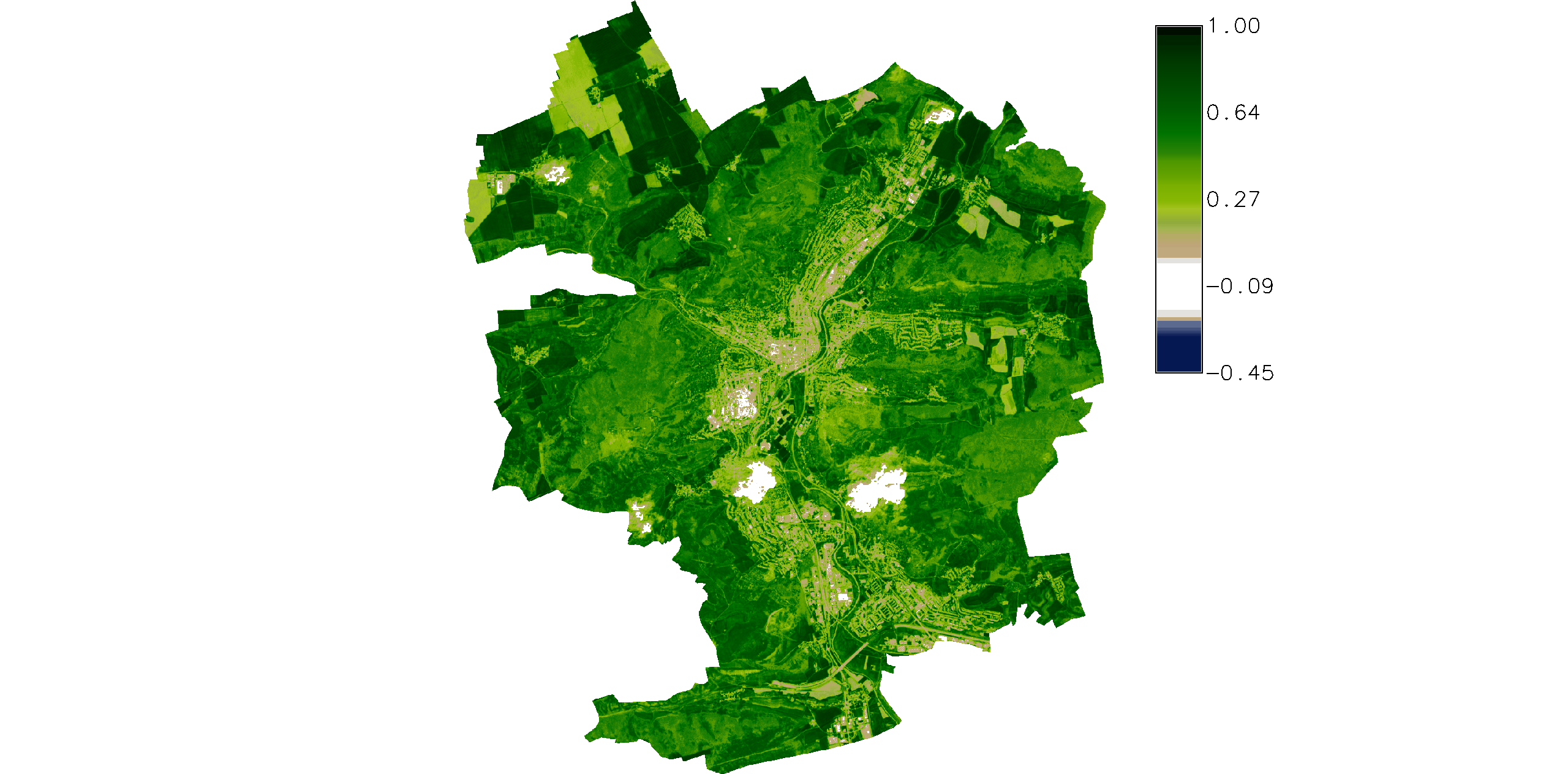
Fig. 110 Simple NDVI animation with clouds masks applied. Computation is limited to AOI only.